Dream RSI: Can Past Discovery Runs Teach an Agent How to Search?
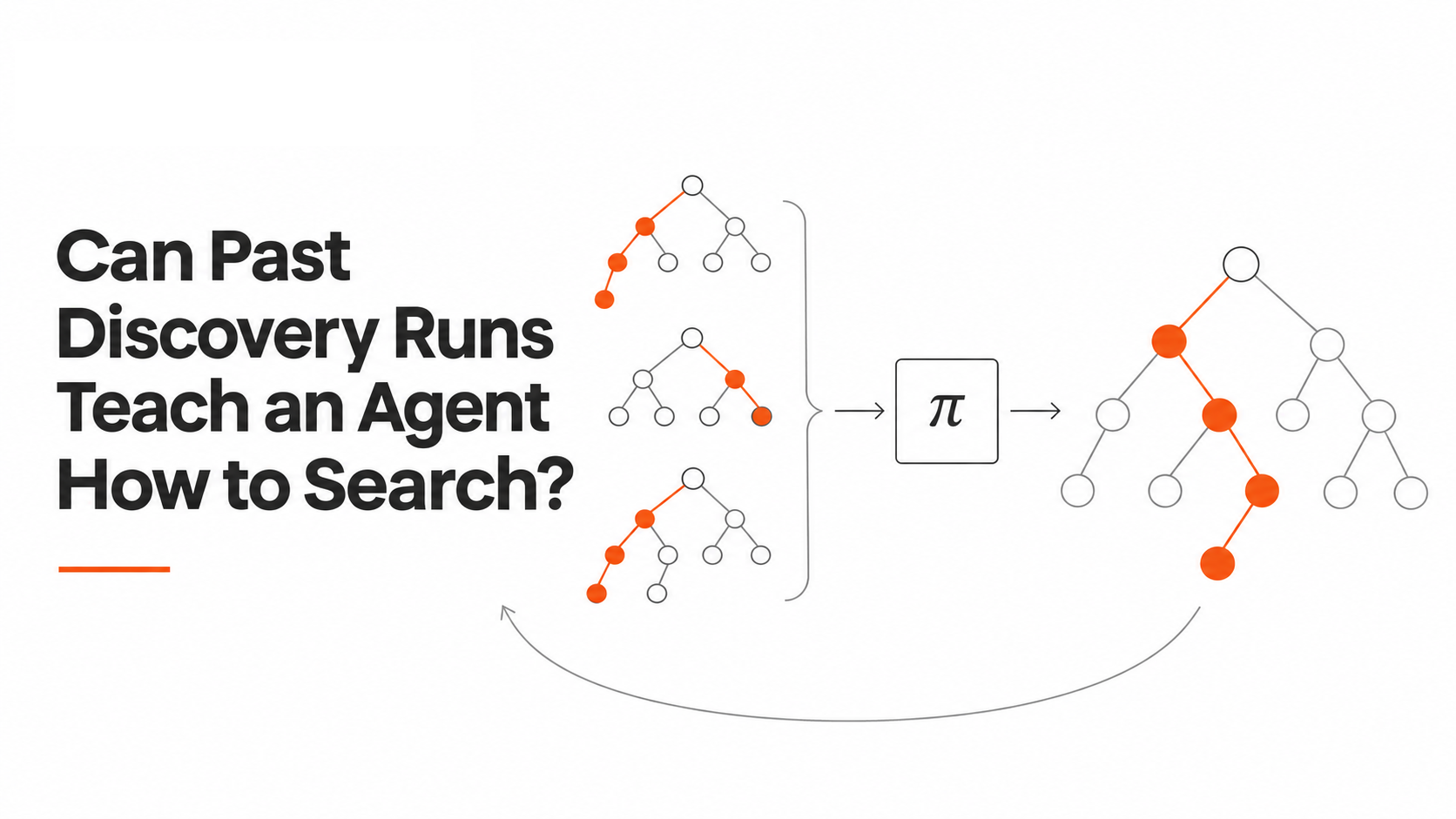
Automated discovery systems such as AlphaEvolve run a simple loop: a coding agent proposes a program, an evaluator scores it, and the result shapes the next proposal. On hard targets, this loop runs for thousands of cycles.
Those cycles must be allocated. Which candidate should be refined next? How many directions should stay open? When should a stagnant branch be dropped? An exploration policy makes these decisions, and it is usually hand-written and fixed.
Improving that policy is hard. A candidate program is scored in minutes, but a policy only reveals its quality after a full run that may cost hundreds of agent calls.
Dream-RSI (Zheng et al., Google and collaborators; arXiv preprint, v2 of 6 October 2026) proposes a shortcut. A recorded run already contains the outcome of every attempt it made, so an alternative policy can be "replayed" over it without calling the agent again.
This article asks: can a recorded discovery history serve as a reliable test bed for exploration policies, and what exactly does it measure?
How a Discovery Tree Becomes a Simulator
Recursive self-improvement, or RSI, refers to systems that improve the procedures producing their own improvements. Dream-RSI targets a narrow layer: not model weights or the coding agent, but the code that schedules the agent's work.
A discovery run is recorded as a tree. The root \(r\) is the initial workspace. Each other node is one attempt, storing its code, diagnostics and score \(s_v\). At each round, the policy picks a batch \(C\) of nodes to continue from:
\[ \begin{gathered} A(\mathcal{T}) = \{r\} \cup \{\, v \in \mathcal{T} : v \text{ is a leaf} \,\} \\ C \subseteq A(\mathcal{T}), \quad |C| \leq W \end{gathered} \]
Here, \(\mathcal{T}\) is the current tree, \(A(\mathcal{T})\) the eligible nodes, and \(W\) the number of parallel workers. Selecting a leaf extends its branch by one attempt; selecting the root opens a new branch. A tree is therefore a set of parallel refinement lines.
Online, each selected node triggers a real attempt by the agent. Offline, the same choice simply reveals the recorded child of that node. Scoring a policy on a recorded tree thus costs only bookkeeping, and one expensive run supports many cheap evaluations.
An analogy helps. A team with a complete lab notebook can ask whether abandoning a line of experiments earlier would have reached its best result sooner, without running anything. But the notebook cannot say what an experiment never run would have produced.
The paper compares this to Dreamer-style world models in reinforcement learning. The mechanism differs: Dreamer learns a generative model that can imagine unseen states, while Dream-RSI looks up recorded outcomes. In our reading, it is closer to off-policy evaluation from logged data.
What the Replay Score Rewards
Each policy is replayed under five budget preferences \(\rho \in \{0, 0.25, 0.5, 0.75, 1\}\), from frugal to patient. This yields points of the form (calls used, quality reached), with quality normalized by the tree's best recorded score. The replay score is:
\[ V_i^m = H_i^m - \lambda\, P_i^m \]
Here, \(H_i^m\) is the area under the quality–cost frontier of policy \(m\) on tree \(i\): reaching high quality with few calls covers more area. \(P_i^m\) is the average number of sequential rounds per call, which is 1 for a serial policy and approaches \(1/W\) when every round fills all workers. The weight \(\lambda\) is not reported in the version we reviewed.
The penalty is a proxy for wall-clock time: identical choices can have very different latency if one policy waits for each result before launching the next.
A small illustration with invented numbers: on a tree of 12 attempts whose best scores 0.70, policy A deepens the leading branch and peaks at 0.56; policy B keeps a weaker branch alive and reaches 0.70 with one call fewer. B scores higher (0.570 versus 0.520 with \(\lambda = 0.1\)). Run serially, B's choices drop to 0.507, below A. No agent call is needed to compute any of this.
The improvement loop
After each online round, a language model, the policy-development agent, reads the replay trajectories and rewrites the policy code three times. The current policy and its three revisions are scored by their average replay score over all recorded trees, and the best is deployed for the next run.
Because the current policy is a candidate, the selected one is never worse on replay. That guarantee says nothing about live performance. Only the policy code changes; the discovery agent and evaluator stay fixed.
What Replay Cannot See
Every replayed outcome is real, so there is no modeling error. That is also the method's boundary. Four limits follow; the first is part of the authors' design, the others are our reading.
Support. A policy can only be scored on attempts that exist. Replay evaluates reallocations of past work, not new exploration, and it does not choose which ideas new branches pursue.
Selection bias. Recorded trees come from earlier policies. A policy that would pursue branches its predecessors abandoned finds little evidence in its favor.
Schedule invariance. Replay assumes an attempt would produce the same result whenever it was made. In live runs, the agent is instructed to read all sibling attempts before proposing, so an attempt's content depends on what other branches had revealed. The paper does not measure this bias.
Cost accounting. Discovery cost counts the coding agent's calls. The policy-development agent's calls are not included, and we did not find them reported.
What the Experiments Show
The controlled baseline, Recursive Fixed Exploration, uses the same agent, evaluator, budget and starting policy, but never revises the policy. Both methods are identical in round one. Cost is measured in cumulative discovery-agent calls. The paper does not report repeated runs or confidence intervals for these tasks.
Lasso regularization path
The agent must write a fast solver for the Lasso, a linear model with an \(\ell_1\) penalty, across a sequence of penalty strengths, matching scikit-learn's objective within \(10^{-6}\). Solvers are timed on six held-out datasets. The last column is our addition: the geometric mean, which weights datasets equally.
| Method | Agent | Calls | RCV1 (ms) | Mean (ms) | Geo. mean (ms) |
|---|---|---|---|---|---|
| SimpleTES (reported) | gpt-oss-120b | 51,200 | 19625.6 | 3804.8 | 121.3 |
| Fixed Exploration | Gemini 3.1 Pro | 550 | 19550.1 | 3587.1 | 159.1 |
| Dream-RSI | Gemini 3.1 Pro | 317 | 14616.0 | 2931.0 | 179.4 |
| Fixed Exploration | Gemini 3.7 Flash | 3200 | 13873.0 | 2516.7 | 127.6 |
| Dream-RSI | Gemini 3.7 Flash | 1879 | 12923.4 | 2350.6 | 117.9 |
Source: Zheng et al., arXiv:2609.14858v2, Figure 4(a). Geometric means computed by Polynom.
Established result. With both agents, Dream-RSI lowers mean runtime while using about 40% fewer calls, and all Gemini solvers beat scikit-learn and glmnet on every dataset.
Error analysis. The mean is dominated by RCV1, the largest dataset. With Gemini 3.1 Pro, Dream-RSI is faster only on RCV1 and slower on the other five; by geometric mean it is slower than its baseline. With Gemini 3.7 Flash, it improves on five of six datasets. The headline 162-fold call reduction versus SimpleTES compares different models, which the authors acknowledge.
Mathematics, kernels and harnesses
Mathematical optimization. Dream-RSI reports the best sum–difference score in the table, ties five other entries on circle packing, and trails its own baseline slightly on autocorrelation. Differences sit in the third to sixth decimal place. These results indicate competitiveness, not a consistent benefit of adaptation.
GPU kernels. On four KernelBench tasks, the controlled comparison consistently favors Dream-RSI: comparable performance with 2.43 and 1.79 times fewer generations on VGG16 and LayerNorm, and 2.09 and 1.44 times higher performance at similar budgets on ConvDiv and ConvMax. This is the strongest evidence for policy adaptation. The best ConvDiv kernel uses 16-bit inputs and is specialized to the benchmark's exact input shape.
Harness optimization. On Terminal-Bench 2.1, the discovered harness scores 0.809, up from 0.725. There is no fixed-policy control, because the authors estimate it would cost over $100,000, and we found no held-out split. The result shows the pipeline works, not that replay caused the gain.
Ablations, all on ConvDiv. Injecting history as prompt hints instead of replaying it lowers performance for both methods. Replaying all past runs instead of only the latest raises performance by 19% but uses 83% more calls: a different trade-off rather than a strict improvement.
Implications for Real Systems
Log runs as structured trees. Storing each attempt with its parent, workspace, score and cost turns every run into a reusable evaluation asset.
Separate the scheduler from the generator. An explicit exploration policy with a narrow interface can be regression-tested on past runs before deployment, with or without a self-improvement loop.
Use replay as a screen, not a verdict. It cheaply discards weak policies, but promising ones still need live confirmation.
Conclusion
Can past discovery runs teach an agent how to search? Within clear limits, yes. A recorded tree is an essentially free simulator for allocation decisions: how deep to pursue branches, how much to parallelize, and when to stop. In controlled comparisons, policies improved this way often match or beat the baseline with fewer calls, most clearly on GPU kernels.
The main limitation is built in. Replay can only reorder what was already tried, and it assumes results do not depend on timing, which does not strictly hold when agents read each other's history. The broader open question is how to evaluate a scheduling policy from logs produced by another policy, with the bias corrections and uncertainty estimates that off-policy evaluation in reinforcement learning has developed.
Sources
Based on arXiv:2609.14858v2 (revised 6 October 2026). Version 1 (14 September 2026) covered eight tasks in three domains and used a different formal replay objective.
- T. Zheng et al. Dream-RSI: Recursive Self-Improvement through Evolving Worlds. arXiv:2609.14858v2, 2026. Code: github.com/zhengkid/Dream-RSI.
- H. Ye et al. Evaluation-Driven Scaling for Scientific Discovery (SimpleTES). arXiv:2604.19341, 2026.
- A. Ouyang et al. KernelBench: Can LLMs Write Efficient GPU Kernels? arXiv:2502.10517, 2025.
- D. Hafner et al. Mastering Diverse Domains through World Models (DreamerV3). arXiv:2301.04104, 2023.